Hand Written Digit Recognizer Using MNIST Dataset

Recently, I’ve been working on the Digit Recognizer (Image Classification) using the MNIST dataset. To say the least, it’s been pretty overwhelming but captivating with numerous previously unknown subject matter. This article is more of a logbook for my-future-self. So, here we go….

About the MNIST database

The MNIST Database (Modified National Institute of Standards and Technology database) is a large database of handwritten digits that is commonly used for training various image processing systems.

alt text

This data set consists of hand drawn numbers from 0 to 9. Each image is 28x28 pixels, for a total of 784 pixels in total. Each pixel has a single pixel-value associated with it, indicating the lightness or darkness of that pixel, with higher numbers meaning darker. This pixel-value is an integer between 0 and 255, inclusive.

Data Preparation

The digits in MNIST dataset have been size-normalized and centered in a fixed-size image. It is a good database for people who want to try learning techniques and pattern recognition methods on real-world data while spending minimal efforts on preprocessing and formatting. But to use the data for the model we have to follow a few steps,

Load and check data
Normalization
Reshape
Train test split

Load and check the data

To ensure that no data corruption occurs during download or reading from csv file

import pandas as pd
train = pd.read_csv('/train.csv')  
test = pd.read_csv('/test.csv')

X = train.drop('label', axis=1)
Y = train['label']

X.isnull().any().describe()
count       784
unique        1
top       False
freq        784
dtype: object

Check if the data is balanced or not (comparing the total dataset for equal distribution of labled data)

import seaborn as sns
sns.countplot(Y) 

alt text

Reshape

Now, we reshape the data in 3 dimensions to represent an image:

-1 keeps the number of data as it, values convert the dataframe to arrays
28, 28 is height and width
1 is grayscale, if we have coloured we should use 3.

X = X.values.reshape(-1, 28,28,1)
test = test.values.reshape(-1,28,28,1)

Train test split

We had two csv files: train.csv and test.csv. But we need a validation dataset to evaluate the model predictions and learn from mistakes. It helps us to tune the model’s parameters depending on the frequent evaluation results on the validation set. So we split the training data set into two portions, 70% train data and 30% validation data hence the test_size=0.3 and the random_state=42 to ensure that the splits that we’ve generated are reproducible. Scikit-learn uses random permutations to generate the splits. The random state that we’ve provided is used as a seed to the random number generator.

from sklearn.model_selection import train_test_split
X_train, X_test, y_train, y_test = train_test_split(X, Y, test_size=0.3, random_state=42)

Normalize

For example, there are different colors such as blue, white, black, so we need to normalize the image to convert the colors to black and white. In short, we can say that we will make that picture in black and white (values between 0 and 1).

This increases the speed of CNN.
The maximum color a picture can take is 255, and we divide this floating by 255.

import tensorflow as tf
x_train = tf.keras.utils.normalize(X_train, axis=1) 
x_test = tf.keras.utils.normalize(X_test, axis=1)

Convolutional Neural Network (CNN)

alt text

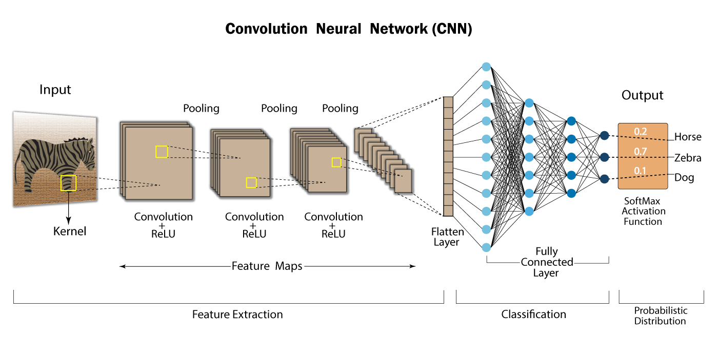
CNN uses their unique properties to distinguish pictures or images. For example: When we look at a cat, our brains use features like ears, tail etc to identify/define the cat, CNN does just that. First, let’s look at its structure before we get started.

Convolutional Layer - Used to determine features
Non-Linearity Layer - Introduction of nonlinearity to the system
Pooling (Downsampling) Layer - Reduces the number of weights and checks fit
Flattening Layer - Prepares data for the Classical Neural Network
Fully-Connected Layer - Standard Neural Network used in classification.

CNN classification uses the normal neural network to solve the problem. However, up to that part, other layers are used to determine the properties.

Convolutional Layer

This layer is the main building block of CNN. It is responsible for perceiving the features of the picture. This layer applies some filters to the image to extract low and high level features in the image. For example, this filter can be a filter that will detect edges.

alt text

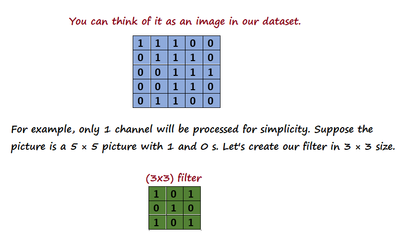
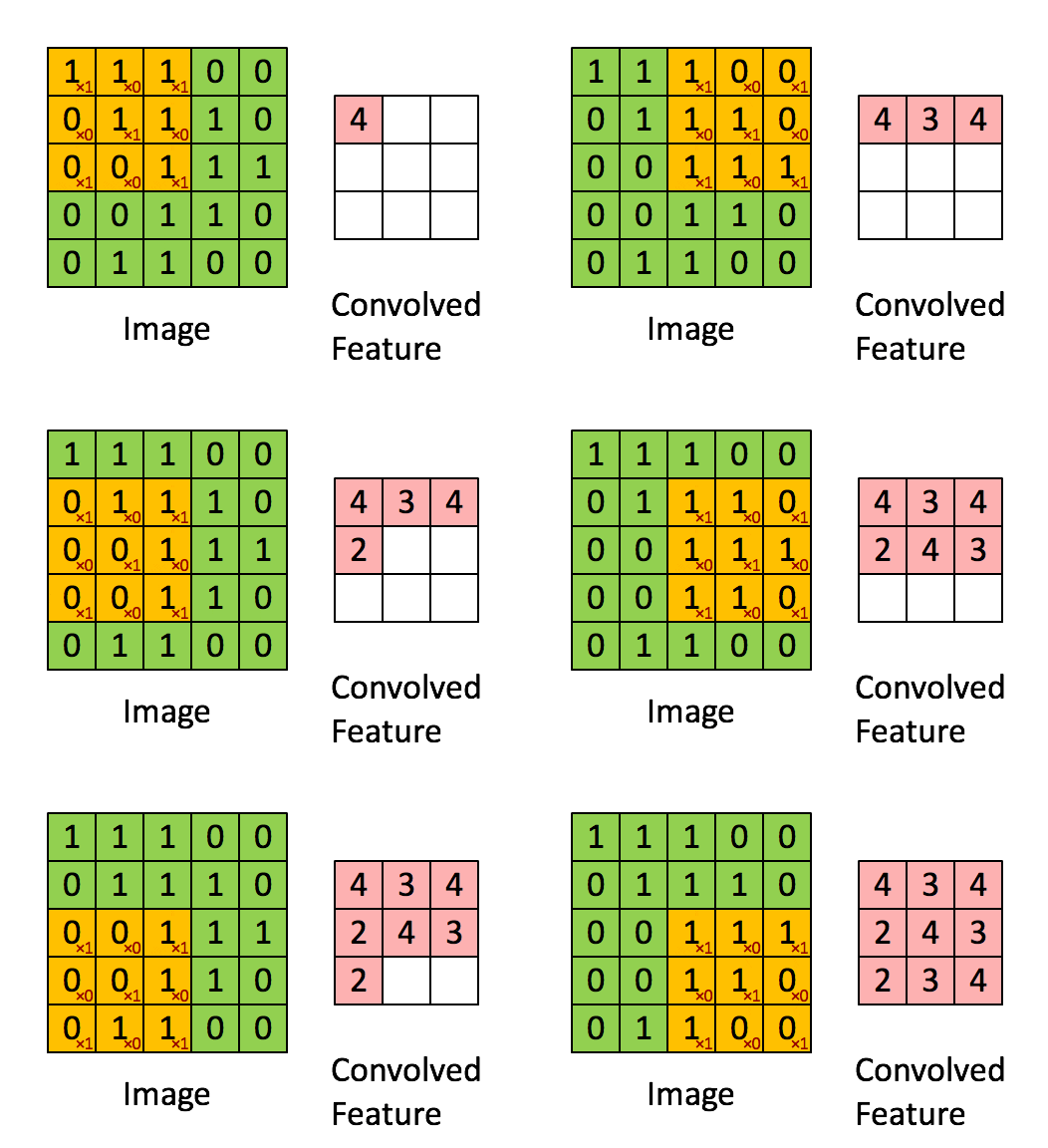
First, the filter is positioned in the upper left corner of the image. Here, the indices between the two matrices (picture and filter) are multiplied by each other and all results are summed, then the result is stored in the output matrix. Then move this filter to the right by 1 pixel (also known as a “step”) and repeat the process. After the end of the 1st line, 2 lines are passed and the operations are repeated. After all operations are completed, an output matrix is created. The reason why the output matrix is 3 × 3 here is because in the 5 × 5 matrix the 3 × 3 filter moves 3 times horizontally and vertically.

Non-linearity

The Non-Linearity layer usually develops after all the Convolutional layers. So why is linearity in the image a problem? The problem is that since all layers can be a linear function, the Neural Network behaves like a single perceptron, that is, the result can be calculated as a linear combination of outputs. This layer is called the activation layer (Activation Layer) because it uses one of the activation functions. [Rectified Linear Unit] (https://www.kaggle.com/dansbecker/rectified-linear-units-relu-in-deep-learning) (ReLU) is one of the most used functions.

alt text

As seen in the picture, ReLU reflects positive inputs as they are, while negative inputs as 0.

alt text

When the ReLu function is applied to the Feature Map, a result as above is produced. Black values in Feature Maps are negative. After the Relu function is applied, the black values are removed and 0 is replaced.

Pooling Layer

This layer is a layer that is often added between successive convolutional layers in ConvNet. The task of this layer is to reduce the shear size of the representation and the number of parameters and calculations within the network. In this way, incompatibility in the network is checked. There are many pooling operations, but the most popular is max pooling. There are also average pooling and L2-norm pooling algorithms that work on the same principle.

alt text

Flattening Layer

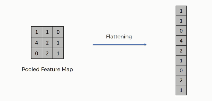
The task of this layer is simply to prepare the data at the input of the last and most important layer, the Fully Connected Layer. Generally, neural networks receive input data from a one-dimensional array. The data in this neural network are the matrices coming from the Convolutional and Pooling layers are converted into a one-dimensional array.

alt text

Fully-Connected Layer

Fully Connected layers in a neural network are those layers where all the inputs from one layer are connected to every activation unit of the next layer. In most popular machine learning models, the last few layers are fully connected layers which compile the data extracted by previous layers to form the final output. It is the second most time consuming layer second to Convolutional Layer.

Note: In this model I’ve only used the flattening layer and Fully-Connected layer. Convolutional layer, Pooling layer weren’t used.

Implementing with keras

Building the model using keras library

# Flatten layer and Fully-Connected layer
model = tf.keras.models.Sequential()
model.add(tf.keras.layers.Flatten())
model.add(tf.keras.layers.Dense(128, activation=tf.nn.relu))
model.add(tf.keras.layers.Dense(128, activation=tf.nn.relu))
model.add(tf.keras.layers.Dense(10, activation=tf.nn.softmax))

# Model compile
model.compile(optimizer='adam',
            loss='sparse_categorical_crossentropy',
            metrics=['accuracy'])

# Fit the model
model.fit(x_train, y_train, epochs=10)Epoch 1/10

919/919 [==============================] - 3s 3ms/step - loss: 0.6223 - accuracy: 0.8232
Epoch 2/10
919/919 [==============================] - 2s 3ms/step - loss: 0.1519 - accuracy: 0.9536
Epoch 3/10
919/919 [==============================] - 2s 3ms/step - loss: 0.0990 - accuracy: 0.9684
Epoch 4/10
919/919 [==============================] - 2s 3ms/step - loss: 0.0695 - accuracy: 0.9784
Epoch 5/10
919/919 [==============================] - 3s 3ms/step - loss: 0.0448 - accuracy: 0.9847
Epoch 6/10
919/919 [==============================] - 3s 3ms/step - loss: 0.0345 - accuracy: 0.9887
Epoch 7/10
919/919 [==============================] - 3s 3ms/step - loss: 0.0266 - accuracy: 0.9915
Epoch 8/10
919/919 [==============================] - 2s 3ms/step - loss: 0.0218 - accuracy: 0.9928
Epoch 9/10
919/919 [==============================] - 2s 3ms/step - loss: 0.0152 - accuracy: 0.9955
Epoch 10/10
919/919 [==============================] - 2s 3ms/step - loss: 0.0147 - accuracy: 0.9944
<tensorflow.python.keras.callbacks.History at 0x7fe5170fb160>

More about this can be found in the keras documentation.

Evaluate the model

The model is evaluated with the 30% train data previously splitted as test data

val_loss, val_acc = model.evaluate(x_test, y_test)
print(val_loss, val_acc)

394/394 [==============================] - 1s 1ms/step - loss: 0.1418 - accuracy: 0.9662
0.14178943634033203 0.9661904573440552

alt text

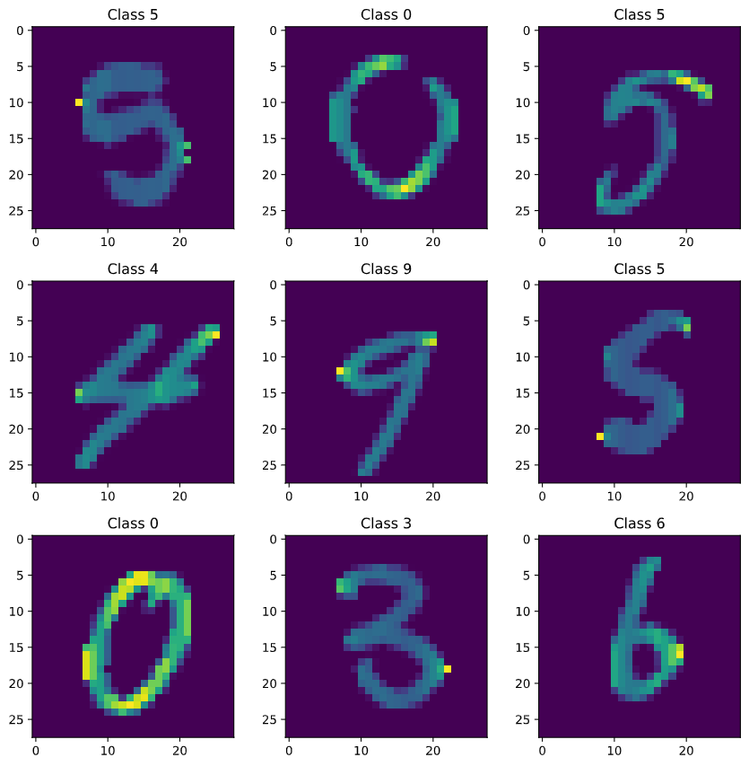
The final evaluation of the model had been tested against the dataset from the test.csv file from which it generated a sample_submission.csv file. It was submitted to the kaggle’s Data Recognizer competition and a score of over 82% was achieved. It’s well enough for this problem as I’ve skipped a few important layers in the CNN. A score of 100% has also been achieved. I should be working on this further to increase the overall score as well as explore a few different approaches.

✨✨ Peace ✨✨

References: