Hand Written Digit Recognizer (MNIST)

21 April 2021 ·4 min read· machine-learning neural-networks mnist tensorflow

A logbook-style writeup of training a small neural network on the MNIST dataset - the classic starting point for image classification. I wrote it as a note to my future self, so it sticks to the parts I needed to reach for later.

About MNIST

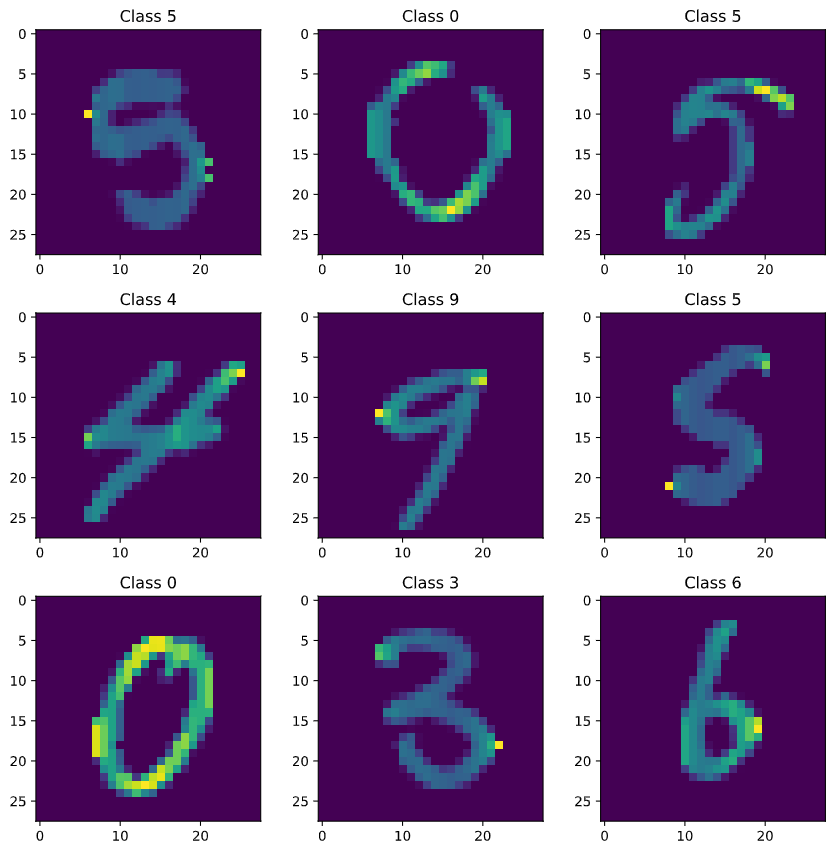
The MNIST database is a large collection of handwritten digits widely used to train and benchmark image processing models. Each image is a 28x28 greyscale grid of pixel values between 0 and 255, where higher values are darker.

Sample training digits

Data preparation

MNIST digits are already size-normalized and centered, so very little cleanup is needed. The workflow:

Load and sanity-check the data.
Confirm label balance.
Reshape into image tensors.
Split into training and validation sets.
Normalize pixel values.

Load and check

import pandas as pd
train = pd.read_csv('/train.csv')
test  = pd.read_csv('/test.csv')

X = train.drop('label', axis=1)
Y = train['label']

A quick X.isnull().any().describe() confirmed there were no missing values across all 784 pixel columns.

Label balance

import seaborn as sns
sns.countplot(Y)

Label distribution

Reshape

MNIST rows are flat 784-pixel vectors. For a CNN we need a 4D shape (samples, height, width, channels):

X    = X.values.reshape(-1, 28, 28, 1)
test = test.values.reshape(-1, 28, 28, 1)

The 1 at the end is the channel count (greyscale). Colour images would use 3.

Train / validation split

from sklearn.model_selection import train_test_split
X_train, X_test, y_train, y_test = train_test_split(
    X, Y, test_size=0.3, random_state=42
)

random_state=42 just makes the split reproducible.

Normalize

import tensorflow as tf
x_train = tf.keras.utils.normalize(X_train, axis=1)
x_test  = tf.keras.utils.normalize(X_test,  axis=1)

Pixel values scale from [0, 255] into [0, 1], which speeds up training and keeps gradients well-behaved.

The model

To keep things simple, this version skipped the convolutional and pooling layers. It’s just a flatten layer followed by fully-connected layers ending in a softmax over 10 classes:

model = tf.keras.models.Sequential()
model.add(tf.keras.layers.Flatten())
model.add(tf.keras.layers.Dense(128, activation=tf.nn.relu))
model.add(tf.keras.layers.Dense(128, activation=tf.nn.relu))
model.add(tf.keras.layers.Dense(10,  activation=tf.nn.softmax))

model.compile(optimizer='adam',
              loss='sparse_categorical_crossentropy',
              metrics=['accuracy'])

model.fit(x_train, y_train, epochs=10)

Training for 10 epochs reached ~99% accuracy on the training set.

Evaluation

val_loss, val_acc = model.evaluate(x_test, y_test)
# loss: 0.1418, accuracy: 0.9662

Sample predictions

The same model, submitted to Kaggle’s Digit Recognizer competition against the held-out test set, scored just over 82%. Stripping the convolutional layers costs accuracy, which is the expected trade-off - adding them back is the obvious next step.